| Transient geotherms |
|||||||||
| Numerical solutions |
|||||||||
 |
|||||||||
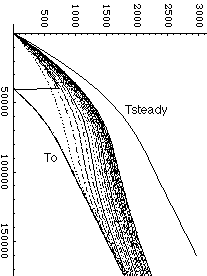
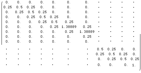
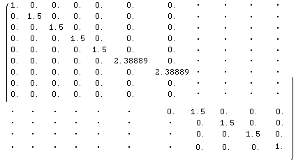
| • We illustrate here a probleme where a continental crust with initial thickness zc is thickened by a factor 2 via the emplacement of one single zt thick thrust. zc=40km, zt=40km. The figure on the right shows the instantantaneous and steady state geotherm (potential geotherm reached after infinite time). The aims is to display transient geotherms down to a depth z=zl+zt at various time intervals, where zl is the thickness of the lithosphere before thickening zl=120km. • We choose a spatial finite diffence h=4000m (spatial grid). Therefore the number of column in the tridiagonal matrixes will be zl/h. The Crank Nicholson scheme imposes the maximum time step of h2/(2.?) = 253,000 years. • We get that Rd=(κ.Δt)/(2h2)=0.25. We assume no erosion: V=0; and we allow for partial melting: Lt=Latent heat/(Cp.(Tliquidus-Tsolidus)). With Rd, V and Lt we can determine ai1, bi1, ci1, the coefficient of the tridiagonal matrix at time n+1, and ai, bi, and ci the coefficient of the tridiagonal matrix at time n. We choose to get the transient geotherm at 20 Myr interval up to 400 Myr. The depth of the tridiagonal matrixes (number of rowl) is therefore 400/20=20. • With this, we construct the tridiagonal coefficient matrixes (7) and (8) , the equation system (7) is solved via matrix inversion (here MatLab and Mathematica are well equiped to do the dirty work...). Graph on the right show transient geotherms from 20 to 400 Ma. |
|||||||||
 |
 |
||||||||
| (7) | (8) | ||||||||
|
|
|
|
|
|
|
|
|
|
|||